Ricky Gill and I have created the R package MittagLeffleR, documented at strakaps.github.io/MittagLeffleR/. It is available on CRAN (and the latest development version on GitHub). MittagLeffleR calculates both Mittag-Leffler distributions; i.e. probability density, cumulative distribution function, quantile function and fast random variate generation. It was made possible by the Laplace inversion algorithm for the Mittag-Leffler function by Roberto Garrappa. Install it via
install.packages("MittagLeffleR")The Two Mittag-Leffler distributions
Various journal articles (including my own) write about “the” Mittag-Leffler distribution, but actually there are two such families of distributions. Both have a shape parameter (tail) taken from the interval \((0,1]\), but the first distribution is very heavy-tailed with infinite mean if tail \(\in (0,1)\) (it is equal to the exponential distribution if tail \(=1\)) whereas the second distribution is light-tailed (has finite moments of all orders). The boolean variable second.type switches between these two distributions.
Examples
First type = waiting times between events
The first type Mittag-Leffler distribution commonly occurs for the inter-arrival times between events in complex systems (e.g. earthquakes, see future post). Suppose that for an event to happen, several “tries” are needed, and that each try has a duration. The number \(N\) of tries until a success is geometrically distributed, and the sum of \(N\) durations is well approximated by a Mittag-Leffler (type I) distribution (this is the geometric stable property).
As an example, we simulate n=100 Mittag-Leffler (type I) random variables, and estimate their tail and scale parameters via maximum likelihood:
library(MittagLeffleR)
y = rml(n = 100, tail = 0.9, scale = 2)
mlml <- function(X) {
  log_l <- function(theta) {
    #transform parameters so can do optimization unconstrained
    theta[1] <- 1/(1+exp(-theta[1]))
    theta[2] <- exp(theta[2])
    -sum(log(dml(X,theta[1],theta[2])))
  }
  ml_theta <- stats::optim(c(0.5,0.5), fn=log_l)$par
  #transform back
  ml_a <- 1/(1 + exp(-ml_theta[1]))
  ml_d <- exp(ml_theta[2])
  return(list("tail" = ml_a, "scale" = ml_d))
}
mlml(y)
## $tail
## [1] 0.9390633
##
## $scale
## [1] 1.600294Second type = number of events
The second type Mittag-Leffler distribution typically occurs for the random number of events in complex systems. For instance, assume a random walk with heavy-tailed waiting times; this has become a widely adopted model for anomalous diffusion. For late times, its number of steps can be well approximated by a Mittag-Leffler (type II) distribution.
The time-change of a random walk by the random number of steps is called subordination; the random number of steps is approximated by the inverse stable subordinator. Below we calculate the probability density of a random walker with step size dx=0.01:
- the number of steps up to time \(t\) is stored in the vector \(h\)
- the matrix \(N\) stores the probability distribution at the lattice sites at consecutive times
- the “subordination” happens in the matrix product
N %*% h.
library(MittagLeffleR)
tail <- 0.65
dx <- 0.01
x <- seq(-2,5,dx)
umax <- qml(p=0.99, tail=tail, scale=1, second.type=TRUE)
u <- seq(0.01,umax,dx)
h <- dml(x=u, tail=tail, scale=1, second.type=TRUE)
N <- outer(x,u,function(x,u){dnorm(x=x, mean=u, sd=sqrt(u))})
p <- N %*% h * dx
plot(x,p, type='l', main="Fractional diffusion with drift at t=1")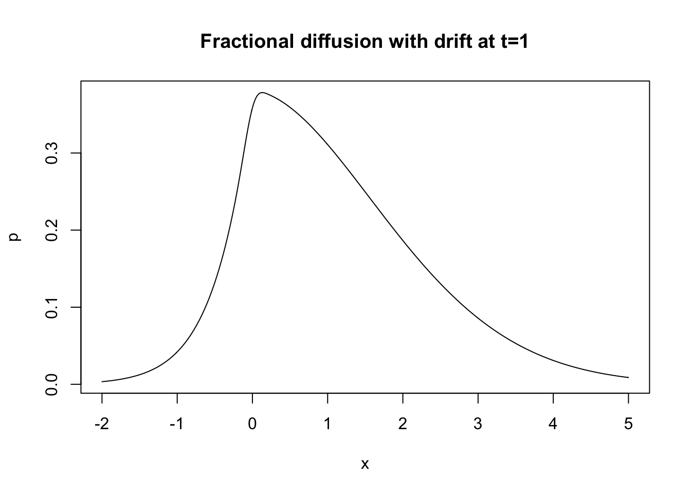
Bugs and Issues
Should you run into any bugs or issues, please let us know. Thanks!