The new R package CTRE is now available on CRAN. “CTRE” stands for “Continuous Time Random Exceedances”, which is a model for extreme values of bursty time series. The theory is desribed in another paper (html|pdf).
library(CTRE)
flares_ctre <- ctre(flares)
plot(flares_ctre, log = "y", main = "Solar Flares")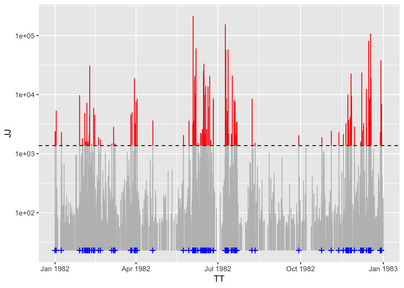
The above time series are measurements of solar flare magnitudes by NASA1. Which observations are considered extreme is defined by a variable threshold \(u\) (dashed line, \(< 5\%\) of observations). The exceedances of this threshold (red) follow (asymptotically for high \(u\)) a Generalized Pareto distribution. This type of modelling of extremes is standard in Extreme Value Theory, and known as the Peaks Over Threshold (POT) method. To date, 18 R packages have been developed for POT!
What’s new about CTRE?
CTRE provides a new way to model the bursty timing of the threshold crossings. In complex systems, inter-event times are typically heavy-tailed2, and thus highly heterogeneous (think income distributions). The bulk of inter-event times is short, corresponding to Bursts of events. A few very long inter-event times represent quiet periods.
The Mittag-Leffler distribution is universal for times between threshold crossings, see the companion paper. CTRE fits a Mittag-Leffler distribution to a range of threshold values:
flares_ctre <- thin(flares_ctre, k = 700)
par(mfrow = c(1,2))
MLestimates(flares_ctre, tail = 0.9, scale = 3E7)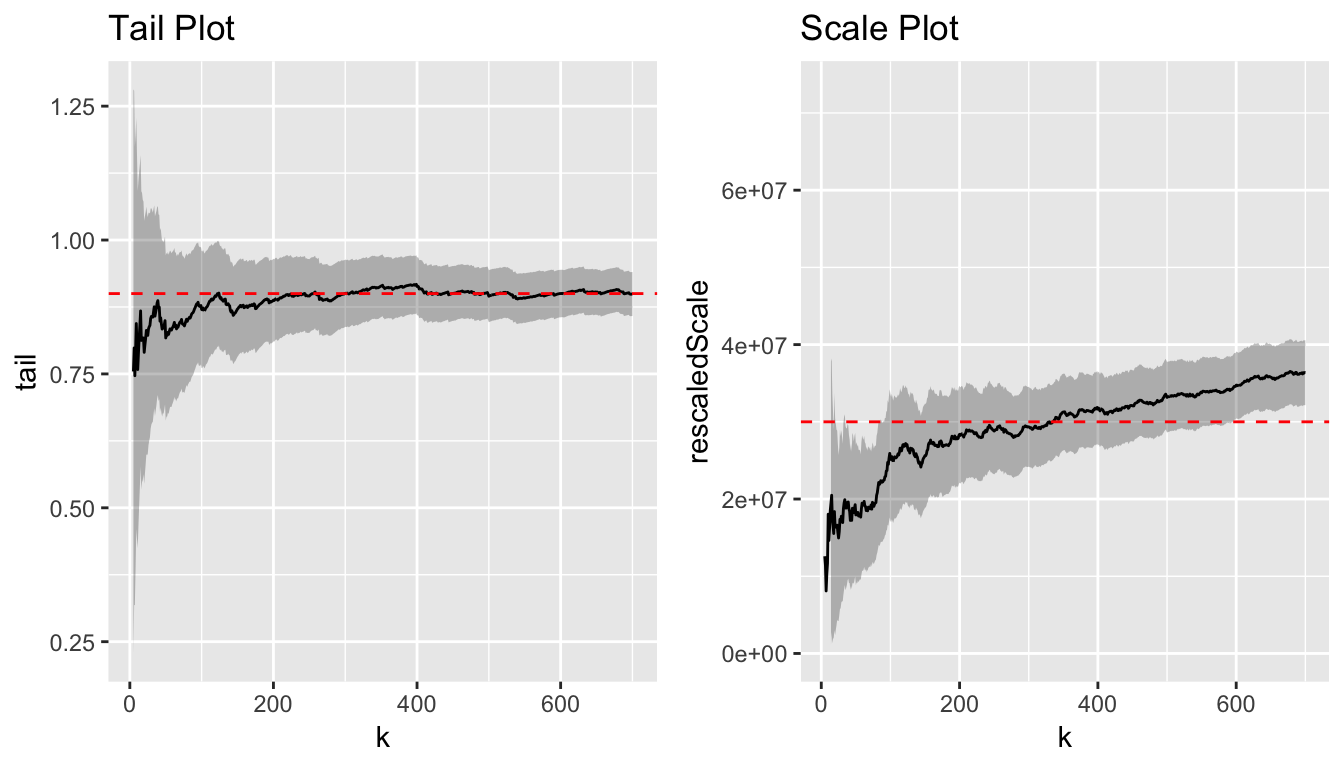
Above, the threshold is varied from the 5th to the 700th largest magnitude (as you move right along the x-axes) and the parameters estimates are plotted on the y-axis. For both panels, towards the left (exceedances=5), only few data are available, and the estimate has a high variance. Towards the right (exceedances = 700), the threshold is low, and the Mittag-Leffler fit degrades (high bias). In between is where we want to read off our (hopefully stable) parameter estimates. The above plots are hence called “stability plots”.
- Important:
The scale parameter is proportional to \(k^{-1/\beta}\). The parameter \(\beta\) is hence used to rescale the y-values of the right-hand plot, in order to make the estimates constant, and needs to estimated from the left-hand plot first.
CTRE applied to data
For the solar flare data, we read off \[ \beta \approx 0.9, \quad \sigma \approx 3 \times 10^7. \] This means that the inter-arrival time \(T(k)\) for magnitudes as high as the \(k\)-th magnitude is distributed as \[ T(k) \sim {\rm ML}\left(0.9, \frac{3 \times 10^7 {\rm sec}}{k^{1/0.9}} \right). \] For example, let’s assume the magnitude (peak rate) \(10,000\). How many magnitudes exceed it?
library(magrittr)
(flares_ctre %>% magnitudes() %>% sort(decreasing=TRUE) > 10000) %>% sum()
## [1] 24So substitute \(k = 24\). The model thus predicts inter-arrival times drawn from the distribution \[ {\rm ML}\left(0.9, 8.8\times 10^{5} {\rm sec} \right) = {\rm ML}\left(0.9, 10 {\rm days} \right). \]
Here’s the plot of this distribution, on a logarithmic scale:
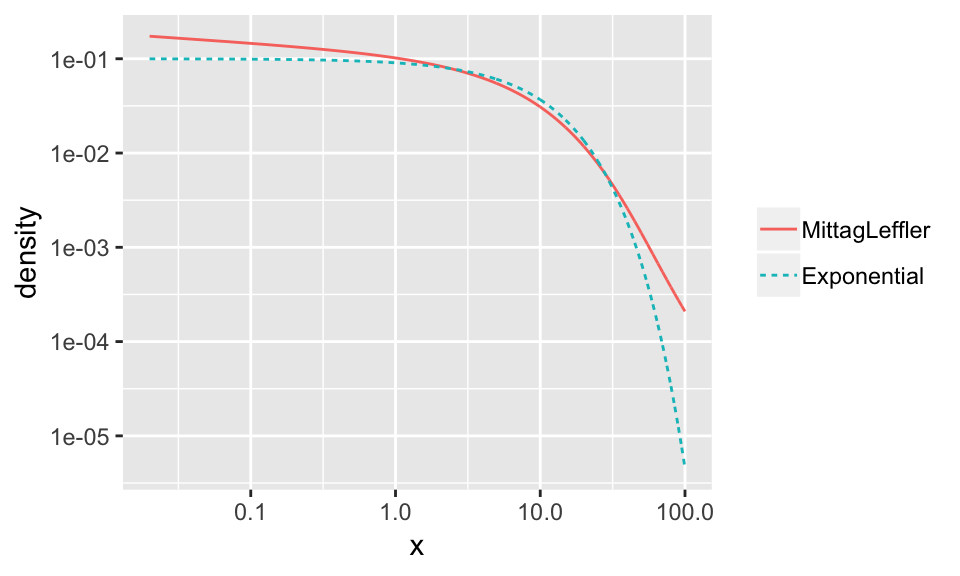
Compared to the Exponential distribution, the Mittag-Leffler distribution puts more probability mass on both tiny values (Bursts) and values in the tails (quiet periods).
Shiny app
Running
CTRE::runCTREshiny()opens a Shiny app that that lets you do the above manipulations via sliders. It is / should be loading below:
What about “clustering of extremes”?
The main other appraoch in Extreme Value Theory which addresses irregular (non-Poissonian) threshold crossing times goes under the name “clustering of extremes”.3 It assumes that the underlying process is stationary, and conflates each excursion of the process above the threshold as one cluster of events.
CTREs and clustering of extremes both generalize the standard assumption of independent events, but in different directions. They are hence complementary, and it needs to be investigated how they should be compared meaningfully.
Feedback
Do you think CTREs are a useful model? Please comment below.
The “complete Hard X Ray Burst Spectrometer event list” is a comprehensive reference for all measurements of the Hard X Ray Burst Spectrometer on NASA’s Solar Maximum Mission from the time of launch on Feb 14, 1980 to the end of the mission in Dec 1989. 12,776 events were detected, with the “vast majority being solar flares”. The list includes the start time, peak time, duration, and peak rate of each event. We have used “start time” as the variable for event times, and “peak rate” as the variable for event magnitudes.↩
See the Introduction of “Modelling bursty time series” by Vajna, Tóth & Kertész, for a list of complex systems with heavy-tailed inter-event times.↩
See e.g. Chapter 3 in the textbook Extremes and Related Properties of Random Sequences and Processes by Leadbetter, Lindgren & Rootzén.↩