An interaction network with many variables

Add Interactions to Regularized Regression

Oct 13, 2018 6 min read statistical learning

Lasso & glinternet

Every Data Scientist and her dog know linear and logistic regression. The majority will probably also know that these models have regularized versions, which increase predictive performance by reducing variance (at the cost of a small increase in bias). Choosing L1-regularization (Lasso) even gets you variable selection for free. The theory behind these models is covered expertly in The Elements of Statistical Learning (for an easier version, see An Introduction to Statistical Learning), and implemented nicely in the packages glmnet for R and scikitlearn for Python.

Few people, however, have heard about glinternet, which is a powerful extension of the Lasso model:

glinternet adds pairwise variable interactions into the Lasso model, and selects these automatically.

It’s a linear model, and thus easily interpretable. Its computational complexity is the same as penalized regression: $\mathcal O(Nm)$ where there are $N$ rows and $m$ variables¹. Thus it handles problems of the same size as (deep) neural networks, potentially with tens of thousands of variables. It should be stressed here that for a thousand variables there are almost 500,000 pairwise interactions that glinternet checks! For structured data, logistic regression is a very useful benchmark model, which can be on par with sophisticated deep learning models even for huge datasets. The glinternet model is more flexible than logistic regression, and is just as interpretable.

A glinternet tutorial

Let’s look at the car90 dataset in the rpart package. It has 25 categorical and 8 continuous predictors, and a continuous outcome (Price). We fit a glinternet model to it, which is a linear model containing all possible pairwise interactions.

Interactions

A linear model without interactions is usually written as

\[y = \beta_0 + \sum_k \beta_k X_k + \varepsilon\]

where $\beta_0$ is the intercept, $X_k$ are predictor variables, $\beta_k$ the coefficients and $\varepsilon$ a model error. We will use categorical variables, so we need to group the variables and coefficients with their categories:

\[y = \beta_0 + \sum_{i=1}^m \sum_{l=1}^{L_i} \beta_{i,l} X_{i,l} + \varepsilon\] where

$m$ is the number of predictors $X_1, \ldots, X_m$
$L_i$ is the number of levels of $X_i$ if $X_i$ is categorical, and 1 otherwise
$(X_{i,1}, \ldots, X_{i,L_i})$ are 0-1 dummy variables representing the categories of $X_i$ (one-hot encoded)

A pairwise interaction model contains all possible pairwise products of the predictors:

\[y = \beta_0 + \sum_{l=1}^{L_i} \sum_{i=1}^m \beta_{i,l}, X_{i,l} + \sum_{1 \le i<j \le m} \sum_{l=1}^{L_i} \sum_{k=1}^{L_j} \theta_{i,j,l,k} X_{i,l} X_{j,k}\]

Interactions, e.g. between variables $X_i$ and $X_j$, occur when the effect of $X_j$ on $y$ will vary depending on the level (or value) of $X_i$. In that case, some of the values $\theta_{i,j, \cdot, \cdot}$ will be non-zero.

Selection of variables and interactions

The L1 regularization is known as the lasso and produces sparsity. glinternet uses a group lasso for the variables and variable interactions, which introduces the following strong hierarchy: An interaction between $X_i$ and $X_j$ can only be picked by the model if both $X_i$ and $X_j$ are also picked. In other words, interactions between two predictors are not considered unless both predictors have non-zero coefficients in the model. The details are in the original paper.

Fitting glinternet

Unfortunately, glinternet’s “API” is not super user friendly… the first challenge is to bring the data into a form that glinternet accepts: The categorical variables need to be (somewhat un-R-like) coded as integers starting from 0. We also need to construct a numLevels vector containing the number of levels $L_1, \ldots, L_m$ in each column if the column is categorical, and 1 else:

library(dplyr)

# Model2 contains model names, which aren't useful here
df <- rpart::car90 %>% select(-Model2)

# drop rows with empty outcomes
df <- df[!is.na(df$Price), ]
y <- df$Price
df <- df %>% select(-Price)

# impute the median for the continuous variables
i_num <- sapply(df, is.numeric)
df[, i_num] <- apply(df[, i_num], 2, function(x) ifelse(is.na(x), median(x, na.rm=T), x))

# impute empty categories
df[, !i_num] <- apply(df[, !i_num], 2, function(x) {
  x[x==""] <- "empty"
  x[is.na(x)] <- "missing"
  x
})

# get the numLevels vector containing the number of categories
X <- df
X[, !i_num] <- apply(X[, !i_num], 2, factor) %>% as.data.frame()
numLevels <- X %>% sapply(nlevels)
numLevels[numLevels==0] <- 1

# make the categorical variables take integer values starting from 0
X[, !i_num] <- apply(X[, !i_num], 2, function(col) as.integer(as.factor(col)) - 1)

A single glinternet model is fitted with the function glinternet; here, we directly fit a 10-fold Cross-Validated model:

library(glinternet)
set.seed(1001)
cv_fit <- glinternet.cv(X, y, numLevels)
plot(cv_fit)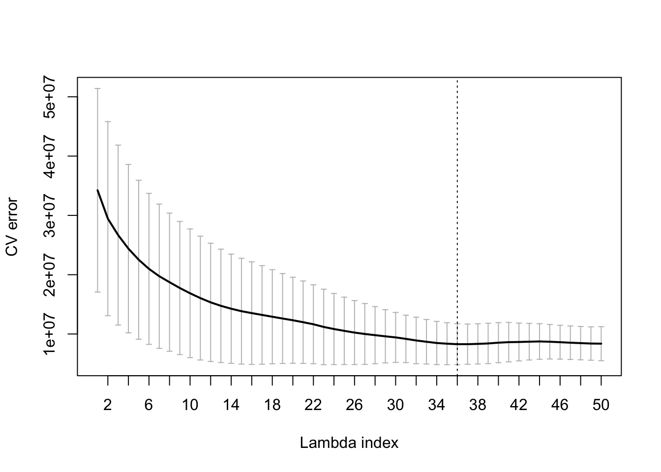

We see the MSE plotted against the decreasing values of regularization parameter lambda.

i_1Std <- which(cv_fit$lambdaHat1Std == cv_fit$lambda)

It is common not to pick the lambda corresponding to the lowest estimate of cross-validation error, but to err on the side of more regularization. So we are happy with a larger lambda with CV error estimate below the minimum plus one standard deviation. This lambda has index i_1Std = 22. Its coefficients $\beta_{i,l}$ and $\theta_{i,j,l,k}$ can be extracted by running

coefs <- coef(cv_fit$glinternetFit)[[i_1Std]]

coefs is a list of 4 items: mainEffects, mainEffectsCoef, interactions and interactionsCoef.

Let’s look at the part without interactions first: The main effects identified are

coefs$mainEffects

## $cat
## [1] 3
## 
## $cont
## [1]  5  7  9 12 20 22 11

which are the indices of the categorical variables and the continuous variables, in order as they occur in the data. We get the indices via

idx_num <- (1:length(i_num))[i_num]
idx_cat <- (1:length(i_num))[!i_num]
names(numLevels)[idx_cat[coefs$mainEffects$cat]]

## [1] "Rim"

names(numLevels)[idx_num[coefs$mainEffects$cont]]

## [1] "Frt.Leg.Room" "Gear.Ratio"   "HP"           "Length"      
## [5] "Tank"         "Weight"       "Height"

The coefficients for these variables are:

coefs$mainEffectsCoef

## $cat
## $cat[[1]]
## [1]    357.6320  -8221.4669   6589.1535 -36595.3391    118.0856   -920.4584
## 
## 
## $cont
## $cont[[1]]
## [1] 35.48628
## 
## $cont[[2]]
## [1] 314.3327
## 
## $cont[[3]]
## [1] -477.2347
## 
## $cont[[4]]
## [1] 9.059015
## 
## $cont[[5]]
## [1] 507.8227
## 
## $cont[[6]]
## [1] 1.366189
## 
## $cont[[7]]
## [1] 104.6502

(I would have expected all of these to be positive; one should check why HP has a negative coefficient.)

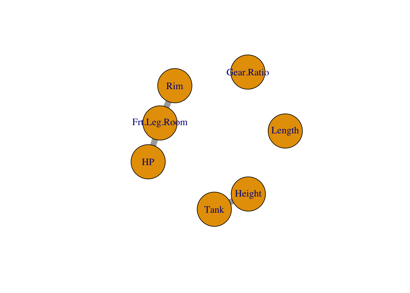
Now for the interaction pairs:

coefs$interactions

## $catcat
## NULL
## 
## $contcont
##      [,1] [,2]
## [1,]    5    9
## [2,]   11   20
## 
## $catcont
##      [,1] [,2]
## [1,]    3    5

The above means:

There is no interaction between the categorical variables (unsurprising because we only identified one. If there was an interaction pair, we would access it via coefs$interactionsCoef$catcat, giving a list of matrices, one matrix of dimension $L_i \times L_j$ for each pair.)
Two pairs of continuous variables have interactions: (5,9) and (11,20), which are (Frt.Leg.Room, HP) and (Height, Tank). The coefficients for these interactions are

coefs$interactionsCoef$contcont

## [[1]]
## [1] 13.66277
## 
## [[2]]
## [1] -6.634724

There is one interaction between categorical variable 3 and continuous variable 5, which are Rim and Frt.Leg.Room. The coefficients for this interaction are:

coefs$interactionsCoef$catcont

## [[1]]
## [1] -164.0751   37.7502 -324.6745  741.9752 -158.0835 -132.8923

Our simple interaction network looks like this:

The model has a root mean squared error (RMSE) on validation data of

sqrt(cv_fit$cvErr[[i_1Std]])

## [1] 3411.904

Compare to linear regression

To quantify how much interactions have contributed to predictive power, we now fit a glmnet model. The best CV mean-squared error for the glmnet model is higher than the mean-squared error for glinternet:

df$Price <- y
X <- model.matrix(Price ~ . - 1, df)
library(glmnet)
cv_glmnet <- cv.glmnet(X,y)
sqrt(min(cv_glmnet$cvm))

## [1] 4238.202

Take-home message

When you’re using logistic or linear regression with Lasso regularization as a baseline, and your next step is to see if adding interactions improve predictive power: try glinternet!

References

Learning Interactions via Hierarchical Group-Lasso Regularization. Michael Lim & Trevor Hastie

Though for this to be true, I believe you have to limit the “interaction search space” via the screenLimit parameter.↩

R Machine Learning